(āpāXāÅü[āhé╠ō³Ś═éŚvŗüé│éĻé▄éĘé¬üAēĮéÓō³Ś═éĄé╚éóé┼EnterāLü[éē¤éĄé─éŁéŠé│éóüBé╗é╠īŃüAé╚é╔é®āTü[āoü[é╔É┌æ▒éĄéĮŚlÄqéÓé╚éŁÄ®Ģ¬é╠āRāōāsāģü[ā^ü[é╠āvāŹāōāvāgé¬ī╗éĻé▄éĘé¬üAé╗éĻé┼éÓcvsé¬ōŁéóé─éóé▄éĘ)ü@é╗é▒é┼üAÄ®Ģ¬é╠āRāōāsāģü[ā^ü[é╠ /usr/tmp/tutorial directory é╔āRā}āōāhé┼ł┌éĶé▄éĘüBé╗éĄé─
Ĥéō³Ś═:ü@ü@ü@ü@ü@ü@ cvs co VSTutorial
éĘéķéŲÄ®ō«ōIé╔ÅŃŗLé╠éµéżé╚āfāBāīāNāgāŖ鬏ņɼé│éĻĢKŚvé╚ātā@āCāŗé¬ā_āEāōāŹü[āhé│éĻé▄éĘüBÄäé╠ÅĻŹćé═æÕø{é┼é═¢│ŚØé┼éĄéĮé╠é┼üAÄ®æŅé┼Ä└ŹséĄé▄éĄéĮé¬üAéRéOĢ¬ł╚ÅŃé®é®é┴éĮéµéżé╔Ävéóé▄éĘüBÅIéĒé┴éĮéń
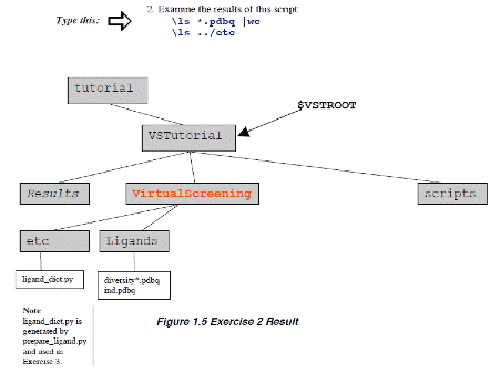
cd VSTutorial
ls
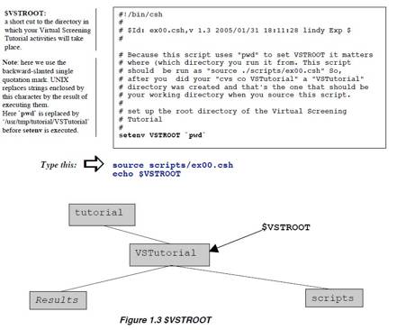
.éŲō³Ś═éĄé▄éĘüBéĘéķéŲüAVSTutorialātāHāŗā_ü[é╔ResultsātāHāŗā_ü[éŲscriptsātāHāŗā_ü[é¬Ä”é│éĻé▄éĘüBĤé╔üAVSTROOTŖ┬ŗ½ĢŽÉöé╠É▌ÆĶééĄé▄éĘüB
>csh
>source scripts/ex00.csh
>echo
$VSTROOT
éŲō³Ś═éĘéķéŲüA/Users/your
account name/tutorial/VSTutorialéŲĢ\Ä”é│éĻéķé═éĖé┼éĘüBEx00.cshāXāNāŖāvāgé╠ōÓŚeé¬ē║ŗLé╠éµéżé╔é╚é┴é─éóéķé®éńüACāVāFāŗé╔éµéĶVSTROOTé╔ŹņŗŲééĄé─éóéķātāHāŗā_ü[¢╝é¬æŃō³é│éĻé▄éĘüB
 ü@
ü@
:
FAQ – Frequently Asked Questions
1. What
library should I use for screening?
If you
want to try and find novel compounds, you probablywant to use a
library designed for diversity, one which probesa large üechemical space.üf If there are small
molecules whichare known to bind to your macromolecule, you may want toconstruct
a tailored library of related compounds.
2. How
much computational time should be invested in each compound? How many dockings,
how many evaluations?
It depends on your receptor and on
the computational resources available to you. One recent successful AutoDock
Virtual Screening used 100 dockings with 5,000,000 evaluations per docking per
compound
.
3. How
do I know which docking results are üehitsüf?
When the results are sorted by
lowest-energy, the compounds which bind as well as your positive control or
better can be considered potential hits. (Remember to allow for the
~2.1kcal/mol standard error of AutoDock). If you have no positive control,
consider the compounds with the lowest energies as potential hits
.
4. Whatüfs
the best way to analyze the results?
Sort them by lowest energy first, then use ADT to inspect
the quality of the binding.
5. Will
I need to visualize the results with the best energies?
Generally it is wise to inspect the
top 30 to 50 results. Some people advocate visually inspecting the top 100-400
hits.
6. What
should I look for when I visualize a docked compound ?
The first thing to check is that
the ligand is docking into some kind of pocket on the receptor. The second is
that there is a chemical match between the atoms in the ligand and those in the
receptor. For example, check that carbon atoms in the8ligand are near
hydrophobic atoms in the receptor while nitrogens and oxygens in the ligand are
near similar atoms in the binding pocket. Check for charge complementarity.
Check whatever else you may know about your particular system: for instance, if
you know that the enzymatic action of your protein involves a particular
residue, examine how the ligand binds to that residue. In the case of HIV
protease, good inhibitors bind in a mode which mimics the transition state.
7. Where can
I get help? The AutoDock mailing list is a good place to start. Informationü@about it and other
AutoDock resources can be found on the AutoDock Web site:
http://www.scripps.edu/mb/olson/doc/autodock
.
Ś¹ÅKü@éP: āŖāKāōāhātāHāŗā_ü[éųpdbātā@āCāŗé╠Åæé½Ź×é▌: sdf to pdb
āoü[ā`āāāŗāXāNāŖü[ājāōāOé╔ŚpéóéķāēāCāuāēāŖé═üAæIé╬éĻéĮāŖāKāōāhātā@āCāŗé®éńɼé┴é─éóéķüBāēāCāuāēāŖī╣é═üAMaybridge (www.maybridge.com), MDL
Mentor, Available Chemicals (UW-Madison)üANCI é┼éĀéķüBāēāCāuāēāŖé═üAé╗é╠āåājü[āNɽüAæĮŚlɽüAé©éµéčłŃ¢“ɽé╔éµéĶæIé╬éĻé─éóéķüBłŃ¢“ɽé═üALinpskyé╠üuéTé╠āŗü[āŗüv üiRule of Fiveüjé╔ŖŅé├éóé─é©éĶüAĢ¬ÄqŚ╩<500üAlogP <5üAÉģæfīŗŹćāhāiü[Éö<5 üAÉģæfīŗŹćāAāNāZāvā^ü[Éö< 10 éŲéóéżŗKæźé╔ł╦é┴é─æIæé│éĻé─éóéķüBāēāCāuāēāŖé╠āTāCāYé═üAÄgŚpē┬ö\é╚āRāōāsāģü[ā^Äæī╣é╔éµéĶæIæéĘéķé▒éŲé¬ÅoŚłéķüBōTī^ōIé╚āēāCāuāēāŖé═üAÉöÉńé╠ātā@āCāŗÆåé®éńÉöÅ\é®éńÉöĢSé¬æIé╬éĻé─éóéķüBŗÉæÕé╚ē╗Ŗwāfü[ā^āxü[āXéāeāXāgéĘéķé▒éŲé═üAÄ└Ź█ōIé┼é═é╚éóüBāēāCāuāēāŖé═üAāŖāKāōāhé╠æĮŚlɽé╔Å┼ō_ééĀé─üAŚŪéóüuhitsüvéÉČé▐ā`āāāōāXéŹ┼æÕé╔éĘéķéµéżé╔Ź\Æzé│éĻéķüB
NCI
Diversity Set āhāēābāOé╠ŖJöŁéæŻÉiéĘéķéĮé▀é╔üANational
Cancer Instituteü@(NCI) é═üA140,000ł╚ÅŃé╠Źćɼē╗ŹćĢ©éŲ80,000ł╚ÅŃé╠āiā`āģāēāŗāvāŹā_āNāgé╠āŖā\ü[āXéł█ÄØéĄüAhigh-through-put screening (HTS)é╔æ╬éĘéķāTāōāvāŗéŚpłėéĄé─éóéķüBNCI Diversity Seté═üAæSé─é╠āŖā\ü[āXé®éńæIé±éŠ1990é╠Ź\æóōIé╔ł┘é╚éķē╗ŹćĢ©é┼éĀéķüB
Babel É╗¢“ŖųīWé┼é╠āŖāKāōāhāēāCāuāēāŖé╠ĢWÅĆātā@āCāŗé═üAsdf (MDL Isis)é┼éĀéķüBāIü[āvāōā\ü[āXāvāŹāOāēāĆé╠babelé═üAÄĒüXé╠ā^āCāvé╠ātā@āCāŗéĢŽŖĘéĘéķāvāŹāOāēāĆé┼éĀéķüBāTā|ü[āgé│éĻé─éóéķā^āCāvé╠āŖāXāgé═üAbabel –méŲéĘéķéŲāüājāģü[āéü[āhé┼babeléÄ└ŹséĘéķüBŹ┼Åēé╠Ś¹ÅKé┼é═üAbabeléÄgéóüAsdfātā@āCāŗé®éń100
pdbātā@āCāŗéÆŖÅoéĄüAAutoDockToolsé╠āXāNāŖāvāgé┼ŚśŚpé┼é½éķéµéżé╔éĘéķüB
Documentationü@ é╗éĻé╝éĻé╠āXāeābāvéŹ─ī╗é┼é½éķÅ┌Źūé╚āhāLāģāüāōāgéŗLŹ┌éĄé─é©éŁé▒éŲé═ĢKÉ{é┼éĀéķüBü@ README ātā@āCāŗé═üAłĻö╩ōIé╚āhāLāģāüāōāgé╠ātā@āCāŗé┼éĀéķüB
āRāōāsāģü[ā^ü[é╔éµéķÄ└ÅKé╠READMEātā@āCāŗé╠ÅdŚvé╚ĢöĢöé╔é═ł╚ē║é╠ŹĆ¢┌é¬Ŗ▄é▄éĻéķüFProject,
Author, Date, Task, Data sources, Files in this directory, Output files,
Running Scripts and other notes on the location of the executable and
environmental settings.ü@ üeBefore We
Startüf āZāNāVāćāōé╔é═üA¢{Å═é┼ÄgŚpéĘéķō³Ś═ātā@āCāŗéŲÄ└ŹsāXāNāŖāvāgéāZābāgāAābāvéĄé─é©éŁüB
æĆŹņ:
1.
ex01.csh
é┼é═üAVirtualScreeningāfāBāīāNāgāŖéŲüAāTāuāfāBāīāNāgāŖLigandséŲetcéŹņɼéĄüAæOÄęé╔é═ŚpłėéĄéĮāŖāKāōāhātā@āCāŗéĹö[éĄüAīŃÄęé╔é═éQüCéRé╠ĢųŚśé╚ātā@āCāŗéō³éĻéķüBĤé╔üAbabeléÄgéóligand.listé╔éĀéķ~100ü@pdb ātā@āCāŗéÆŖÅoéĄĢŽŖĘéĘéķüBé▒éĻéńé═üANCI
Diversity Set éŖ▄é▐diversity.sdf é®éńÆŖÅoéĘéķüBŹ┼īŃé╔üAā|āWāeāBāuāRāōāgāŹü[āŗéŲéĄé─ind.pdbéé╗é╠āfāBāīāNāgāŖé╔Ģ█æČéĘéķüB
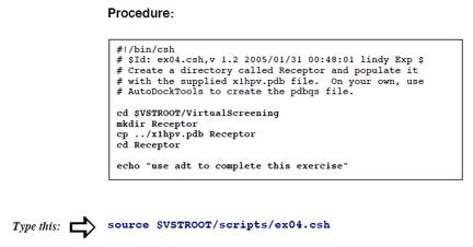
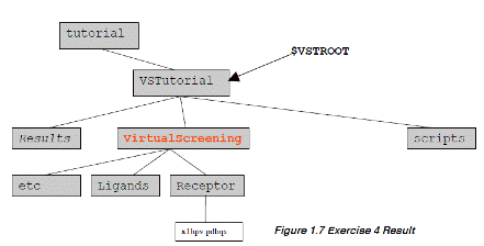
Ś¹ÅKéQ: āŖāKāōāhātā@āCāŗé╠ĢŽŖĘ: pdb to pdbq.
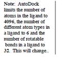
AutoDock experiment é═üAō┴ÆĶé╠ī¤Ź§ŗ¾Ŗįé┼é╠āxāXāgüiŹ┼żé╠āGālāŗāMü[éÄØé┬üjé╠āRāōātāHāüü[āVāćāōéÄ”éĘīŗŹćāŖāKāōāhŹ\æóéĢ\Ä”éĘéķüBAutoDock experiment é╔æ╬éĘéķō³Ś═ātā@āCāŗé╔é═üAAutoDocké╔éµéĶāTā|ü[āgé│éĻéķī┤Äqā^āCāvāZābāgé╔éĀéķī┤Äqł╚ŖOé═Ŗ▄é▄éĻé─é═é╚éńé╚éóüBé▒é╠āZābāgé╔é═üAunited-atom aliphatic carbons, aromatic carbons in cycles, polar
hydrogens, hydrogen-bonding nitrogens éŲüAĢöĢ¬ōdēūéÄØé┐üAæ╝é╠ī┤ÄqéŲÆ╝É┌ÉģæfīŗŹćéĄé─éóéķÄ_æféŖ▄é▐üB
AutoDock é╠ōKÉ│é╔Źņɼé│éĻéĮō³Ś═ātā@āCāŗé═üAAutoDock é╠ī┤Äqā^āCāvāZābāgéŲłĻÆvéĄé─éóéķī┤Äqé╔æ╬éĘéķpdbé╔ÄŚéĮāīāRü[āhé®éńé╚éķüBé╗é╠ātā@āCāŗé╠Źņɼé╔é═īćæ╣éĄé─éóéķī┤ÄqéŌōYē┴ÉģüAéQĢ¬Äqł╚ÅŃé╠Ģ¬ÄqüAŹĮé╠ÉžÆfüAalternate locationé╔éµéķā|āeāōāVāāāŗÉöé╠¢ŌæĶéēīłéĘéķé▒éŲéÓŖ▄é▄éĻé─éóéķüB
¢{ā`āģü[āgāŖāAāŗé┼é═üAāOāēātāBāJāŗāCāōā^ü[ātāFü[āXé┼éĀéķADTéŚpéóé─üAāŖāKāōāhātā@āCāŗéŹņɼéĘéķüBēĮÉńéÓé╠āŖāKāōāhātā@āCāŗéGUIé╔éµéĶŹņɼéĘéķé▒éŲé═üAéĀé▄éĶæ├ō¢é╚ŹņŗŲéŲé═īŠé”é╚éóüBé╗é╠éµéżé╚ŹņŗŲé═Ä®ō«ē╗é│éĻéķĢKŚvé¬éĀéĶüA¢{Å═é┼é═üAAutoDockTools é╔éĀéķāpāCā\āōāXāNāŖāvāgé┼éĀéķprepare_ligand.pyéÅąēŅéĄUNIXé╠foreach loopÆåé┼é╠ÄgŚp¢@é╔é┬éóé─ÅqéūéķüBÅ┌Źūé═ AppendxéÄQÅŲéĄé─éŁéŠé│éóüB
æĆŹņ
ü@
3. Document:
READMEātā@āCāŗé╔é▒é╠āZāNāVāćāōé╠ŹĆéē┴é”éķüBīxŹÉé╠āüābāZü[āWéŗLś^éĘéķüBé▒é╠Ś¹ÅKé┼é═éPéOé╠āCāōāvābāgātā@āCāŗé¬ügNot all ligand written:ühéŲéóéżīxŹÉéÅoŚ═éĄé─éóéķüBUNIXé╠üescript filenameüfāRā}āōāhé═READMEātā@āCāŗéĢŽŹXéĘéķĢ╩é╠Ģ¹¢@é┼éĀéķüBé╗é╠āRā}āōāhé═ÄwÆĶé│éĻéĮātā@āCāŗé╔ā^ü[ā~āiāŗé╔ÅoŚ═é│éĻéĮéĘéūé─é╠āeāLāXāgéāRāsü[éĘéķüBé▒é▒é┼é═üAé╗é╠āgāēāōāXāNāŖāvāgéforeachāŗü[āvé╠æOé╔ŖJÄnéĄüAControl D é╔éµéĶÅIéĒéńé╣éķüB
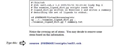
Ś¹ÅKéR: Profiling the library: ī┤ÄqÄĒāZābāgé╠īłÆĶ
āŖāZāvā^ü[é╔æ╬éĘéķāŖāKāōāhé╠āhābāLāōāOéÄÄé▌éķŹ█é╔üAAutoDocké═āŖāZāvā^ü[é╠ō┴ÄĻé╚Ģ\ī╗ī^üAüugrid mapsüvéŲī─éįgrid-based potential energies ātā@āCāŗéÄgŚpéĘéķüBAutoGridé═üAāhābāLāōāOé╔ŚpéóéķāŖāKāōāhÆåé╠æSī┤ÄqÄĒé╔æ╬éĄé─łĻé┬é╠grid
mapéīvÄZéĘéķüBāOāŖābāhā}ābāvé═ŗKæźōIé╔āŖāZāvā^ü[é╠ijéĶé╔özÆué│éĻéĮéRDŖiÄqéµéĶé╚éĶüAō¢ŖYé╠ā}āNāŹĢ¬Äqé╠ŗ╗¢ĪéÄØé┴é─éóéķö═ł═é╔é╗é╠ÆåÉSéÆuéŁüBé╗éĻé╝éĻé╠āOāŖābāhā}ābāvé╠ā|āCāōāgé═üAā}āNāŹĢ¬Äqé╠ī┬üXé╠ī┤ÄqéŲō┴ł┘é╚āvāŹü[āuī┤ÄqéŲé╠āyāAé┼é╠ā|āeāōāVāāāŗæŖī▌ŹņŚpé╠Źćīvé┼éĀéķüB'n'ī┬é╠ŖłÉ½āgü[āVāćāōé┼īłé▀éńéĻéĮāOāŖābāhā}ābāvé┼āJāoü[é│éĻéĮéRDé╠ŚeÉŽé═üAéUü{'n'ī┬é╠search spaceéÆĶŗ`éĘéķüB
éPī┬é╠āŖāZāvā^ü[é╔æ╬éĘéķāŖāKāōāhé╠āZābāgé╠āhābāLāōāOé┼é═üAī┬üXé╠āŖāKāōāhÆåé╔æČŹ▌éĘéķī┤Äqā^āCāvé╠covering
setÆåé╔éĀéķŖeī┤Äqā^āCāvé╔éĮéóéĄé─łĻī┬é╠āOāŖābāhā}ābāvé¬ĢKŚvé┼éĀéķüBé▒é╠āGāNāTāTāCāYé┼é═ī┤Äqā^āCāvé╠covering
setéīłé▀üAŚ]éĶé╔éÓæĮéóī┤ÄqüAī┤Äqā^āCāvüAē±ō]ē┬ö\é╚ā{āōāhé╚éŪéÅ£ŖOéĘéķéĮé▀é╔āŖāKāōāhāēāCāuāēāŖé╠Śv¢±éŗLś^éĘéķüB
æĆŹņ:
 éŪé╠ī┤ÄqÄĒé¬æ╬Å█é╔é╚é┴é─éóéķé®éÆŹłėéĘéķüBé╗é╠ÅŅĢ±Ä¤æµé┼é═üAéóéŁé┬é®é╠īnŚ±éĵéĶÅ£éŁĢKŚvé¬éĀéķüB
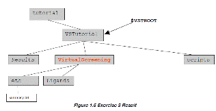
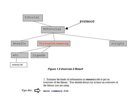
. 2.ü@āēāCāuāēāŖéŖTŖŽéĘéķéĮé▀é╔é═üAsummary.txtÆåé╠ÅŅĢ±éā`āFābāNéĘéķüBÅĒé╔Ägé┴é─éóéķāēāCāuāēāŖéŖTŖŽéĘéķé▒éŲé═ÅdŚvé┼éĀéķüB

2.
é▒é╠āZāNāVāćāōé╠æĆŹņé╠āGāōāgāŖéREADME ātā@āCāŗé╔ē┴é”é─é©éŁüB
ÆŹüFŚßé”é╬ī¤Åoé│éĻéĮī┤ÄqÄĒüAāgü[āVāćāōÉöé╠ö═ł═é╚éŪ
.
ü@
Ś¹ÅKéS: āŖāZāvā^ü[é╠ÅĆö§: pdb épdbqsé╔ĢŽŖĘ.
AutoDocké┼ŚpéóéķāŖāZāvā^ü[ātā@āCāŗé═ā`āāü[āWüfqüféŲŚnö}śaāpāēāüü[ā^üfsüfüiAtVol, the atomic
fragmental volume, éŲ AtSolPar, the atomic solvation parameterü@éŖ▄é▐üjépdbé╔ē┴é”éĮpdbqsātāHü[ā}ābāgé┼é╚é»éĻé╬é╚éńé╚éóüBAtVol éŲAtSolPar é═ā}āNāŹĢ¬Äqé╠āŖāKāōāhīŗŹćé╔éµéķŚnö}é╠Å£ŗÄé╔ł╦æČéĄéĮāGālāŗāMü[éīvÄZéĘéķé╠é╔ŚpéóéķüBAutoDockü@atom types éŖmöFéĘéķéĮé▀é╔üAŗ╔ɽÉģæfé¬æČŹ▌éĄé╚é»éĻé╬é╚éńé╚éóéĄüAö±ŗ╔ɽÉģæféŲīŪŚ¦ōdÄqæ╬é¬ē┴é”éńéĻé╚é»éĻé╬é╚éńé╚éóüBé│éńé╔üAæSé─é╠ī┤Äqé═Kollmané╠ĢöĢ¬ā`āāü[āWéŖäéĶō¢é─üACNOSHł╚ŖOé╠ī┤Äqé╔ŖųéĄé─é═üAāÅāCāŗāhāJü[āhé┼éĀéķüfXüfé®üfMüféŲéĄé─ÄwÆĶé│éĻé╚é»éĻé╬é╚éńé╚éóüBæSé─é╠ÄcŖŅé╔ŖųéĄé─é═üAintegural total chargeé¬ŖäéĶō¢é─éńéĻéķüB
āŖāZāvā^ü[ātāHāŗā_ü[é═üAāŖāZāvā^ü[éłĻōxéŠé»ÅłÆuéĘéķātāHāŗā_ü[é┼éĀéķüBéĘéūé─é╠āŖāKāōāhé═é▒é╠łĻé┬é╠āŖāZāvā^ü[é╔æ╬éĄé─ÅłÆué│éĻéķüBAutoDockTools tutorial ātāHāŗā_ü[é®éńÄ└Źsé┼é½éķéŲĢųŚśé┼éĀéķüB
ü@
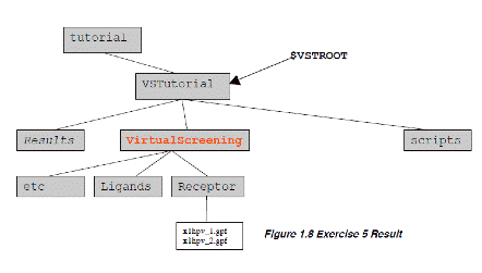
Ś¹ÅKéT: āēāCāuāēāŖé╠éĮé▀é╠AutoGridāpāēāüü[ā^ātā@āCāŗé╠Źņɼ
ü@āOāŖābāhāpāēāüü[ā^ātā@āCāŗé═üAAutoGridé╔æ╬éĄé─īvÄZéĘéķā}ābāvé╠ā^āCāvüAé╗é╠ā}ābāvé╠éĀéķÅĻÅŖéŌæÕé½é│éÄwÆĶéĄüAłĻægé╠ā|āeāōāVāāāŗāGālāŗāMü[āpāēāüü[ā^éō┴ÆĶéĘéķüBłĻö╩é╔üAłĻé┬é╠ā}ābāvé═āŖāKāōāhÆåé╠é╗éĻé╝éĻé╠āGāīāüāōāgéŲÉ├ōdōIā}ābāvé╔æ╬éĄé─īvÄZé│éĻéķüBÄ®ī╚¢ĄÅéé╠é╚éó12-6 Lennard-JonesāGālāŗāMü[āpāēāüü[ā^üARij,ĢĮŹtÄ×ŖjŖįŗŚŚŻüAāGālāŗāMü[ŗ╔żÆl(well
depth)é¬ā}āNāŹĢ¬Äqé╠ī┤Äqā^āCāvé╔ŖŅé├éóé─é╗éĻé╝éĻé╠ā}ābāvé╔æ╬éĄō┴ÆĶé│éĻéķüBÉģæfīŗŹćéāéāfāŗē╗éĄéĮéóÅĻŹćé═üAgpfé╠12-6āpāēāüü[ā^é╠æŃéĒéĶé╔12-10āpāēāüü[ā^éō┴ÆĶéĘéķé▒éŲé┼é╗éĻéÄ└ŹséĘéķüBāŖāKāōāhé╠āēāCāuāēāŖłĻé┬é╔æ╬éĄé─üAāŖāKāōāhé╠łĻé┬é╠ī┤Äqā}ābāvé¬ĢKŚvé┼éĀéķüBé╗éĻé╝éĻé╠AutoGridé╠īvÄZé┼éUī┤Äqā}ābāvéŲÉ├ōdā}ābāv鬏ņéńéĻéķüBÅ]é┴é─üAāŖāōāKāōāhāēāCāuāēāŖé╔æ╬éĘéķAutoGridé╠æŹÄdÄ¢Éöé═üAāēāCāuāēāŖÆåé╠ī┤Äqā^āCāvé╠Éöé╔ł╦æČéĄé─éóéķüBéÄī┬é╠ī┤Äqā^āCāvé¬æČŹ▌éĄé─éóéķéŲüAn/6 + 1é╠āOāŖābāhāpāēāüü[ā^ātā@āCāŗéÅĆö§éĘéķĢKŚvé¬éĀéĶüAAutoGridé═n/6 + 1ē±Ä└Źsé│éĻéķé▒éŲé╔é╚éķüB
ü@
1.
adtéŚpéóé─āOāŖābāhāpāēāüü[ā^ātā@āCāŗ(gpf)éÅæéŁüFüiéÓ饌¹ÅKéSé┼ŚpéóéĮā}āNāŹĢ¬ÄqéÄgéżé╚éńüAé▒é╠Ź┼Åēé╠āXāeābāvé═ĢKŚvé╚éóüj:ü@
* Grid -> Macromolecule -> Openüc(AG3)]ü@
* Grid -> Open GPFücü@
../../x1hpv.gpf éŲā^āCāvéĄüA āNāŖābāN Open
* Grid -> Set Map Types -> Directlyüc(AG3)
ü@ü@ü@ ACHNOS éŲā^āCāvéĄüAāNāŖābāN Accept
* Grid -> Output
-> Save GPFüc(AG3)
ü@ü@Receptor directory é┼x1hpv_1.gpf éŲā^āCāvéĄüAāNāŖābāN Save
* Grid ->
Set Map Types -> Directly..(AG3)
ü@cbFP ā^āCāvéĄüAāNāŖābāN Accept
ü@* Grid -> Output -> Save GPFüc(AG3)
ü@Receptor directory é┼x1hpv_2.gpf éŲā^āCāvéĄüAāNāŖābāN Save.
 2. ŹĪŹņɼéĄéĮō±é┬é╠āOāŖābāhāpāēāüü[ā^ātā@āCāŗéĤé╠éµéżé╔éĄé─āeāXāgéĘéķüB
3. README fileé╔é▒é╠āZāNāVāćāōé╠æĆŹņéē┴é”é─é©é½é▄éĄéÕéż
4. Linux machinesé┼é═, Control Zé╠é┬é¼é╔bg éŲā^āCāvéĄéōāoābāNāOāēāEāōāhé┼é`écéséēęōŁé│é╣é─é©é½é▄éĘüB
ü@
Ś¹ÅKéU: AutoGridéŚpéóé─āŖāKāōāhāēāCāuāēāŖé╔æ╬éĘéķī┤ÄqāAātāBājāeāBā}ābāvéīvÄZéĘéķüB
é▒é╠Ś¹ÅKé╠éµéżé╚āēü[āWāXāPü[āŗé┼é╠āoü[ā`āāāŗāXāNāŖü[ājāōāOīvÄZÄ└ī▒é┼é╠ɼī„ŚvīÅé═üAāfü[ā^é╠ægÉDē╗é┼éĀéķüBé┬é▄éĶüAæĮéŁé╠āCāōāvābāgüAāAāEāgāvābāgātā@āCāŗéægÉDē╗éĘéķéĮé▀é╔Ŗ╚¢Šé╚āfāBāīāNāgāŖŹ\æóéÄgéżĢKŚvé¬éĀéķüBé▒é╠Ś¹ÅKé┼é═üAāŖāZāvā^ü[éōŲŚ¦éĄéĮāfāBāīāNāgāŖé╔Æué½üAé╗é▒é╔éĘéūé─é╠é▒é╠āīāZāvā^ü[é╔æ╬éĄé─īvÄZé│éĻéĮAutoGridāAātāBājāeāBü[ā}ābāvéĢ█æČéĄéĮüBéĘéūé─é╠āŖāKāōāhāfāBāīāNāgāŖé╔é═üAé╗éĻé╝éĻé╠ā}ābāvātā@āCāŗéŲreceptor.pdbqsé╔æ╬éĄé─āVāōā{āŖābāNāŖāōāNéĢ█æČéĄé─éĀéķüBé╗éĻé╝éĻé╠āŖāKāōāhāfāBāīāNāgāŖé╔é═üAé╗é╠ligand.pdbqātā@āCāŗéŲāhābāLāōāOāpāēāüü[ā^ātā@āCāŗé┼éĀéķx1hpv_ligand.dpfé¬Æuéóé─éĀéķüB¢{Ś¹ÅKé┼é═üAautogrid3ééQē±x1hpvé╔æ╬éĘéķĢKŚvé╚ī┤Äqā}ābāvāZābāgéīvÄZéĘéķéĮé▀é╔Ägé┴é─éóéķüBé╗éĻé╝éĻé╠āŖāKāōāhé╔æ╬éĄé─āVāōā{āŖābāNāŖāōāNéŹņɼéĘéķéĮé▀é╔āŖāZāvā^ü[āfāBāīāNāgāŖé┼ŹņŗŲéĘéķüB
Procedure:
2. Check
that the maps are there and check that there are 10 maps
ü@
3. README ātā@āCāŗé╔é▒é╠āZāNāVāćāōé╠æĆŹņéē┴é”é─é©é½é▄éĄéÕéż
Ś¹ÅKéV: ā|āWāeāBāuāRāōāgāŹü[āŗé╔éµéķāvāŹāgāRü[āŗé╠ī¤Åž
Ä└ŚpōIé╚æÕé½é│é╠āŖā\ü[āX鳥éóāoü[ā`āāāŗāXāNāŖü[ājāōāOé╠Ä└ī▒ééĘéķæOé╔üAō³Ś═ātā@āCāŗ鬢ŌæĶé╚éóé®éŪéżé®éī¤ōóéĘéķüB
ü@ü@AutoDockéŚpéóé─āhābāLāōāOééĘéķÅĻŹćüAī┬üXé╠ē▀Æ÷é═ō»éČÅēŖ·ÄĶÅćéōźé±é┼ĢĪÉöé╠āhābāLāōāOē▀Æ÷éÄ└ŹséĘéķüBāhābāLāōāOé╠ÄĒüXé╠āpāēāüü[ā^ü[é═üAĢüÆ╩āhābāLāōāOāpāēāüü[ā^ü[ātā@āCāŗüA"DPF"é╔Ģ█æČé│éĻéķüBé▒é╠ātā@āCāŗé═üAAutoDocké╠āRā}āōāhāēāCāōé┼flagé╔(-p)éé┬é»éķé▒éŲé┼ō³Ś═é│éĻéķüBé╗éĻé╝éĻé╠āŖāKāōāhé═üAō┴ŚLé╠āhābāLāōāOātā@āCāŗéÄgŚpéĘéķüBé▒é╠Ś¹ÅKé┼ÄgŚpéĘéķāhābāLāōāOāpāēāüü[ā^ü[éÅæéŁéĮé▀é╔é═üAprepare_dpf.pyéŲéóAutoDockTools/Utilitiesé╔éĀéķāXāNāŖāvāgéŚpéóéķüBÄgéóĢ¹é╠Å┌Źūé═Appendix é╔ŗLé│éĻé─éóéķüB
 ü@
ü@
Ś¹ÅKéW:āhābāLāōāOātāHāŗā_ü[é╠ŹņɼéŲāēāCāuāēāŖÆåé╠āŖāKāōāhé╗éĻé╝éĻé╔æ╬éĘéķāpāēāüü[ā^ātā@āCāŗé╠Źņɼ
é▒é╠Ś¹ÅKé┼é═üAæOē±é╠Ś¹ÅKé┼āXāNāŖü[ājāōāOé╠ī┬üXé╠āŖāKāōāhé╔ŚpéóéĮāXāeābāvéā|āWāeāBāuāRāōāgāŹü[āŗé╔æ╬éĄé─ŹséżüBé╗éĻé╝éĻé╠āŖāKāōāhé╔æ╬éĄé─ī┬Ģ╩é╠āfāBāīāNāgāŖé¬éĀéķüBé╗éĻé╝éĻé╠āŖāKāōāhé╠āfāBāīāNāgāŖé═autogridā}ābāvé╔éŲāīāZāvā^ü[é╔æ╬éĘéķāVāōā{āŖābāNāŖāōāNéŖ▄é±é┼éóéķüBé╗éĻé╝éĻé╠āŖāKāōāhāfāBāīāNāgāŖé═é│éńé╔üAī┬üXé╠ligand.pdbq éŲ ligand.dpf ātā@āCāŗéŖ▄é±é┼éóéķ.
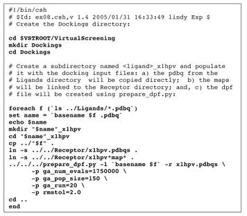 Procedure:
Suggestion: unsetü@echo here ifü@it is set because this scriptü@involves many stepsü@for many ligands.
ü@
3. README ātā@āCāŗé╔é▒é╠āZāNāVāćāōé╠æĆŹņéē┴é”é─é©é½é▄éĄéÕéż
ü@
Ś¹ÅKéX:ĢĪÉöé╠
AutoDock jobé╠Ä└Źs.
üié▒é╠Ä└ÅKé┼é═æOéÓé┴é─īvÄZéĄé─é©éóéĮīŗē╩éŚpéóé▄éĘüBüj
æĆŹņ:
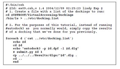
 ex09.cshāXāNāŖāvāgé╠ōÓŚeé═üAé╗é╠ōÓŚeéÄ└ŹséĘéķāRāōāsāģü[ā^é╔éµéĶł┘é╚éĶé▄éĘüBæÕŹŃĢ{Ś¦æÕŖwüEÉČĢ©ÅŅĢ±ē╚Ŗwē╚Ä└ÅKÄ║é┼é═ł╚ē║é╠éµéżé╔Åæé½ŖĘé”é─Ä└ŹséĄé▄éĘüB
echo
"autodock3 -p $d.dpf -l $d.dlg
é╠Źsé
autodock3
-p $d.dpf -l $d.dlg
éŲéĄé▄éĘüBé▒éĻé═üAex09.cshé¬üAŚ¹ÅKé╠éĮé▀é╔éĘé┼é╔īvÄZéĄé─éĀéķīŗē╩éŚpéóéķéµéżé╔ŗLÅqéĄé─éĀéķé®éńé┼üAÄ└Ź█é╔Ä└ŹséĘéķŹ█é═echoéé═éĖéĄé▄éĘüBŗNō«éĄéĮīŃé═üAÄ└ŹsæOé╔
>csh
>limit
stacksize unlimited
éŲéĄé─é©é½é▄éĘüBéĮéŠéĄüAŚ¹ÅKéVé¬éżé▄éŁÄ└Źsé┼é½éĻé╬é▒é╠ŹņŗŲé═Å╚é»é▄éĘüB
ü@2. āhābāLāōāOātāHāŗā_ü[é╔éĀéķāhābāLāōāOāŹāOéā`āFābāNéĄé▄éĘüB:
 ü@3. README ātā@āCāŗé╔é▒é╠āZāNāVāćāōé╠æĆŹņéē┴é”é─é©é½é▄éĄéÕéż
Ś¹ÅK10üFāhābāLāōāOīŗē╩é╠ī¤ōó-īŗŹćāGālāŗāMü[é╠Åćł╩
é▄éĖüAé╗éĻé╝éĻé╠āŖāKāōāhé╔æ╬éĄé─łĻöįÆßéóāGālāŗāMü[é╔éµéķāhābāLāōāOé╠āŖāXāgéŹņɼéĘéķüBé╗é╠éĮé▀é╔üAæSé─é╠āŖāKāōāhé╠NNN.dlgélig_rec.energieséŲéĄé─ŹņɼéĄüAé┬éóé┼é╗é╠ātā@āCāŗéā\ü[āgéĄé─lig_rec.energies.sortéŹņɼéĘéķüB
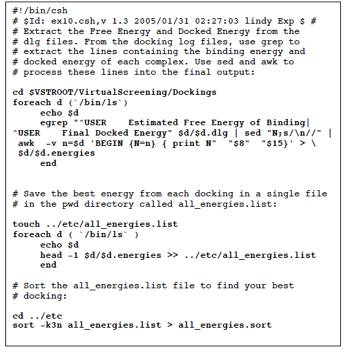
 æĆŹņüF
Note: Docking energy is the sum of the
intermolecular energy plus the internal energy of the ligand. Binding energy is the sum of the intermolecular
energy plus the torsional free energy penalty (0.3113*number of active
torsions) ü@
Note: head -1 puts the single best result
for each ligand into all_energies.list. You could use head -2 or
head -3 to
include more results. Note: -k3n means use field 3 which
is the docking energy. ü@
|
|
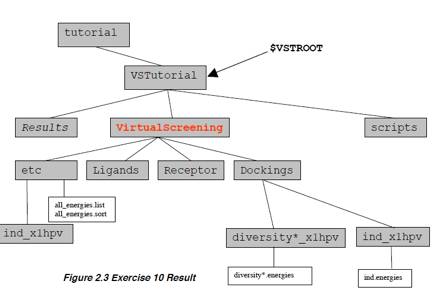
2. īŗē╩é╠ī¤ōóéł╚ē║é╠éµéżé╔éĄé─ŹséżüB
>cd ../Dockings
>head
diversity1988_x1hpv/diversity1988_x1hpv.energies
>pwd
>ls
2. all_energies.sortātā@āCāŗé┼āŖāXāgé╠āgābāvé╔éĀéķŹ┼żāGālāŗāMü[üiŹ┼ŚŪīŗŹćüjé┼īŗŹćéĄé─éóéķāŖāKāōāhéŖmé®é▀éķüBā|āWāeāBāuāRāōāgāŹü[āŗéŲöõŖréĄé─üAé╗éĻł╚ÅŃé╠īŗŹćééĄé─éóéķāŖāKāōāhéāmü[āgéĘéķüB
>cd ../etc
>head all_energies.sort
4. README ātā@āCāŗé╔é▒é╠āZāNāVāćāōé╠æĆŹņéē┴é”é─é©é½é▄éĄéÕéż.
Ś¹ÅK11: Ź┼ōKé╠āhābāLāōāOüEāŖāKāōāhé╠ī¤ōó
1. adt:Ä└Źs
cd ../Dockings
adtüiadté¬āoābāNāOāēāōāhé┼ēęō«éĄé─éóéķÅĻŹćé═fgāRā}āōāhéÄgŚpéĘéķüj
2. vieweré╠āZābāgāAābāv
* File->Preferences->Set
Commands to be Applied on Objects
- Available
commands āŖāXāgé®éń colorByAtomType éæIæ
-ü@ '>>'éāNāŖābāNü@ü@ üFæIæéĄéĮāRā}āōāh鬌ūéųł┌Źs
-ü@ 'OK'éāNāŖābāNü@ü@ üFŖmÆĶ
* File->Browse
Commands
- select a packageāŖāXāgé®éńPmv éāNāŖābāN
- moduleé╠āŖāXāgé®éńbondCommandséæIæ
-Load ModuleéāNāŖābāN
-msmsCommandséæIæ
-Load ModuleéāNāŖābāN
-DISMISSéāNāŖābāN
3. āŖāZāvā^ü[é╠āZābāgāAābāv
* Read in the file:
File->Read
Molecule
ü@ü@ü@ü@ü@ -
"PDB files (*.pdb)" éāNāŖābāN
-"AutoDock files (pdbqs) (*.pdbqs) éæIæ
-"x1hpv.pdbqs"éæIæ
* Set center of rotationüF
ü@ü@ü@ü@ü@ -
pointing finger iconéāNāŖābāN
ü@ü@ü@ü@ü@ -
PCOM levelé®éńMolecule éæIæéĄAtom éāNāŖābāN
ü@ü@ü@ü@ü@ -
"printNodeNames" é╠ēEéāNāŖābāNéĄcenterOnNodes"é
æIæ
-Éģé¬æČŹ▌éĘéķĢėéĶé╔ā{ābāNāXéĢ`éŁ
(PCOM level é¬Atomé╔É▌ÆĶéĄé─éĀéĻé╬ā{ābāNāXé═ē®ÉFé╔é╚éķ)
ü@ü@ü@ü@ü@ü@ü@ü@ * Display msms surface:
Compute->Molecular
Surface->Compute Molecular Surface
ü@ü@ü@ü@ü@ -
MSMS Parameters Panel widgeté┼OKéāNāŖābāN
Color->by Atom Type
ü@ü@ü@ü@ü@ -
MSMS-MOLéāNāŖābāNéĄ
OKéāNāŖābāN
* Make molecular surface
transparent using the DejaVu GUI:
ü@ü@ü@ü@ü@ -
DejaVuGUI (Sphere/Cube/Cone) ButtonéāNāŖābāN
ü@ü@ü@ü@ü@ -
+ rootéāNāŖābāN
ü@ü@ü@ü@ü@ -
+ x1hpvéāNāŖābāN
- MSMS-MOLéæIæ
ü@- Material: FrontéāNāŖābāN
-change Opacity to .7
ü@ü@ü@ü@ü@ -
Material: NoneéāNāŖābāN
- viewer é┼current object éŲéĄé─rootéæIæ
* Close the DejaVu GUI:
ü@ü@ü@ü@ü@ü@ü@ü@ - DejaVuGUI (Sphere/Cube/Cone)éāNāŖābāN
* ADJUST the view:
-ā}āEāXé╠Æåā{ā^āōéSHIFTéē¤éĄé╚é¬éńē¤é│é”é─ō«é®éĄx1hpvüfé╠ÉģéāYü[āĆéĘéķ
4. Repeat the following
steps for each docking to be evaluated. Here
we show the procedure using diversity0619_x1hpv.dlg
as an
example:
1. Analyze->
Docking Logs->Open
-diversity0619_x1hpv.dlgéæIæ
ü@ü@ü@ü@ü@ü@ü@ü@ü@ü@ü@ü@ü@ü@ -
OpenéāNāŖābāN
ü@ü@ü@ü@ü@ü@ü@ü@ü@ü@ü@ü@ü@ü@ -
OKéāNāŖābāN
2. Analyze->
Clusterings->Show
write a printable
version of histogram:
ü@- histogramüfs Edit-> WriteéāNāŖābāN
-type in this
filename: ügdiversity0619_x1hpv.psüh
ü@ü@ü@ü@ü@ü@ü@ü@ü@ü@ü@ü@ü@ü@ -
SaveéāNāŖābāN
3. Visualize the
lowest energy docked conformation
-type üedüf in the viewer to turn off depth-cueing
ü@ü@ü@ü@ü@ü@ü@ü@ü@ü@ü@ü@ü@ü@ -
lowest energy bin in the histogram to open the playeréāNāŖābāN
ü@ü@ü@ü@ü@ü@ü@ü@ü@ü@ü@ü@ü@ü@ -
right arrow to set ligand to 1_1 conformationéāNāŖābāN
Assess:
-is the
ligand in a pocket?
-is each
atom in the ligand in a chemically favorable position?
Show hydrogen bonds:
ü@ü@ü@ü@ü@ü@ü@ü@ü@ü@ü@ü@ü@ü@ -
playerüfs amperes and for play optionséāNāŖābāN
ü@ü@ü@ü@ü@ü@ü@ü@ü@ü@ü@ü@ü@ü@ -
Build H-bonds and
Show InfoéāNāŖābāN
-Record number of
hbonds formed
-Display
Distance(1.741) or Energy(-5.931)
4. Clea n-up for next
docking log
ü@ü@ü@ü@ü@ü@ü@ü@ü@ü@ü@ü@ü@ü@ -
Close on üediversity0619üf widgetéāNāŖābāN
ü@ü@ü@ü@ü@ü@ü@ü@ü@ü@ü@ü@ü@ü@ -
File->Exit on üediversity0619:rms=2.0éāNāŖābāN
clusteringüf histogram
-ü@ü@ü@ü@ü@ü@ü@ü@ü@ü@ü@ü@ü@ü@ü@ü@ü@ü@ü@ü@ü@ü@ü@ Analyze->Dockings->Clear
to delete this docking
5. README ātā@āCāŗé╔é▒é╠āZāNāVāćāōé╠æĆŹņéē┴é”é─é©é½é▄éĄéÕéż
Using
the TSRI (The Scripps Research Institute) cluster: bluefish.
All input file preparation should be done on your local
computer. The interactive head node on the bluefish cluster is used
to transfer the files from your computer to the cluster where the calculations
will be carried out. For todayüfs tutorial, we will demonstrate
launching a sample docking and then use previously computed results.
We create a tar file of the VSTutorial directory tree:
Appendix A: AutoDockTools ScriptsÄgŚp¢@
ü@AutoDockToolsāéāfāģü[āŗ é╔éĀéķprepare_ligand.py āXāNāŖāvāgé═āCāōāvābāgātāēābāOé╔éµéĶāJāXā^āĆē╗ē┬ö\é┼éĀéķüB
Note: You can generate any
of these usage
statements
by typing the
script name
with no input.
eg:
prepare_ligand.py
|
|
prepare_ligand.py –l ligand_filename
[vo:d:A:CKU:B:R:Mh]
-l ligand
filename (required)
Optional
parameters include (defaults are in parentheses):
-v verbose output (none)
-o output pdbq_filename (ligandname.pdbq)
-d dictionary filename to write summary information of per
molecule atomtypes and number of active torsions (none)
-A type(s) of repairs to make (none):
bonds
hydrogens
bonds_hydrogens
-C do not add charges (add gasteiger charges)
-K add Kollman charges (add gasteiger charges)
-U cleanup type, what to merge (nphs_lps)
nphs
lps
üg üg
-B types of
bonds to allow to rotate (backbone)
amide
guanidinium
amide_guanidinium
üg üg
-r root (auto)
index for
root
-m mode
(automatic)
interactive
(do not automatically write outputfile)
The prepare_receptor.py
script in AutoDockTools module isü@customizable via input flags:
prepare_receptor.py
–r filename ['r:vo:A:CGU:M:']
-r receptor_filename
Optional
parameters:"
-v verbose
output
-o pdbqs_filename
(receptor_name.pdbqs)
-A type(s)
of repairs to make (üg üg):
bonds_hydrogens
bonds
hydrogens
-C do not
add charges (add Kollman charges)
-G add
Gasteiger charges (add Kollman charges)
-U cleanup
type, what to merge (nphs_lps)
nphs
lps
üg üg
-m mode (automatic)
interactive (do not
automatically write outputfile)
The prepare_dpf.py
script is customizable via input flag (default
values
are in parenthese)s
:
prepare_dpf.py
-l ligand_filename –r receptor_filename
-l ligand_filename
-r receptor_filename
Optional
parameters:"
-v verbose
output
-o dpf_filename
(ligand_receptor.dpf)
-i template
dpf_filename
-p parameter_name=new_value